aula_4 – <i class='bi bi-graph-up'></i> FIP 606

O que aprendemos?

1. Modelos Lineares com Transformações

Uso de lm() com transformação (ex: sqrt(count))
Comparações com emmeans() e cld()
Avaliação de resíduos com simulateResiduals() do pacote DHARMa

2. Modelos Lineares com Família Poisson (GLMs)

Ajuste com family = poisson
Visualização de resíduos simulados
Médias estimadas com emmeans(..., type = "response")
Diagnóstico com check_model()

3. ANOVA com Dois Fatores e Interação

Uso de lm() com interação ~ fator1*fator2
Visualização com interaction.plot()
Comparações por nível com emmeans() e cld()
Cálculo do coeficiente de variação com cv.model()

4. Cálculo do AUDPC e ANOVA Fatorial

Uso da função AUDPC() do pacote epifitter
Agrupamento com group_by() + summarise()
Ajuste de modelo com dois fatores: irrigation_type e moisture
Interações significativas e interpretação

# Pacotes necessários
library(DHARMa)

This is DHARMa 0.4.7. For overview type '?DHARMa'. For recent changes, type news(package = 'DHARMa')

library(emmeans)

Welcome to emmeans.
Caution: You lose important information if you filter this package's results.
See '? untidy'

library(multcomp)

Carregando pacotes exigidos: mvtnorm

Carregando pacotes exigidos: survival

Carregando pacotes exigidos: TH.data

Carregando pacotes exigidos: MASS


Anexando pacote: 'TH.data'

O seguinte objeto é mascarado por 'package:MASS':

    geyser

library(car)

Carregando pacotes exigidos: carData

library(performance)
library(gsheet)
library(ggplot2)
library(agricolae)
library(epifitter)
library(dplyr)


Anexando pacote: 'dplyr'

O seguinte objeto é mascarado por 'package:car':

    recode

O seguinte objeto é mascarado por 'package:MASS':

    select

Os seguintes objetos são mascarados por 'package:stats':

    filter, lag

Os seguintes objetos são mascarados por 'package:base':

    intersect, setdiff, setequal, union

Modelo Linear com Transformação (sqrt)

InsectsDataframe = InsectSprays
InsectAnovaResult = lm(sqrt(count) ~ spray, data=InsectsDataframe)
M = emmeans(InsectAnovaResult, ~ spray)
cld(M)

 spray emmean    SE df lower.CL upper.CL .group
 C       1.24 0.181 66    0.883     1.61  1    
 E       1.81 0.181 66    1.447     2.17  12   
 D       2.16 0.181 66    1.802     2.53   2   
 A       3.76 0.181 66    3.399     4.12    3  
 B       3.88 0.181 66    3.514     4.24    3  
 F       4.02 0.181 66    3.656     4.38    3  

Results are given on the sqrt (not the response) scale. 
Confidence level used: 0.95 
Note: contrasts are still on the sqrt scale. Consider using
      regrid() if you want contrasts of back-transformed estimates. 
P value adjustment: tukey method for comparing a family of 6 estimates 
significance level used: alpha = 0.05 
NOTE: If two or more means share the same grouping symbol,
      then we cannot show them to be different.
      But we also did not show them to be the same.

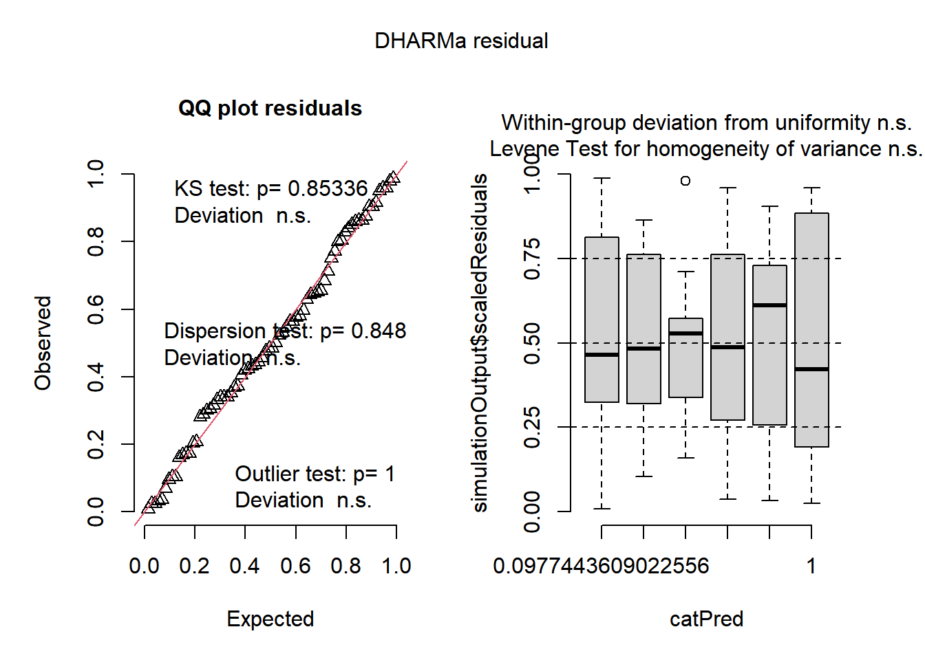
plot(simulateResiduals(InsectAnovaResult))

GLM com Distribuição Poisson

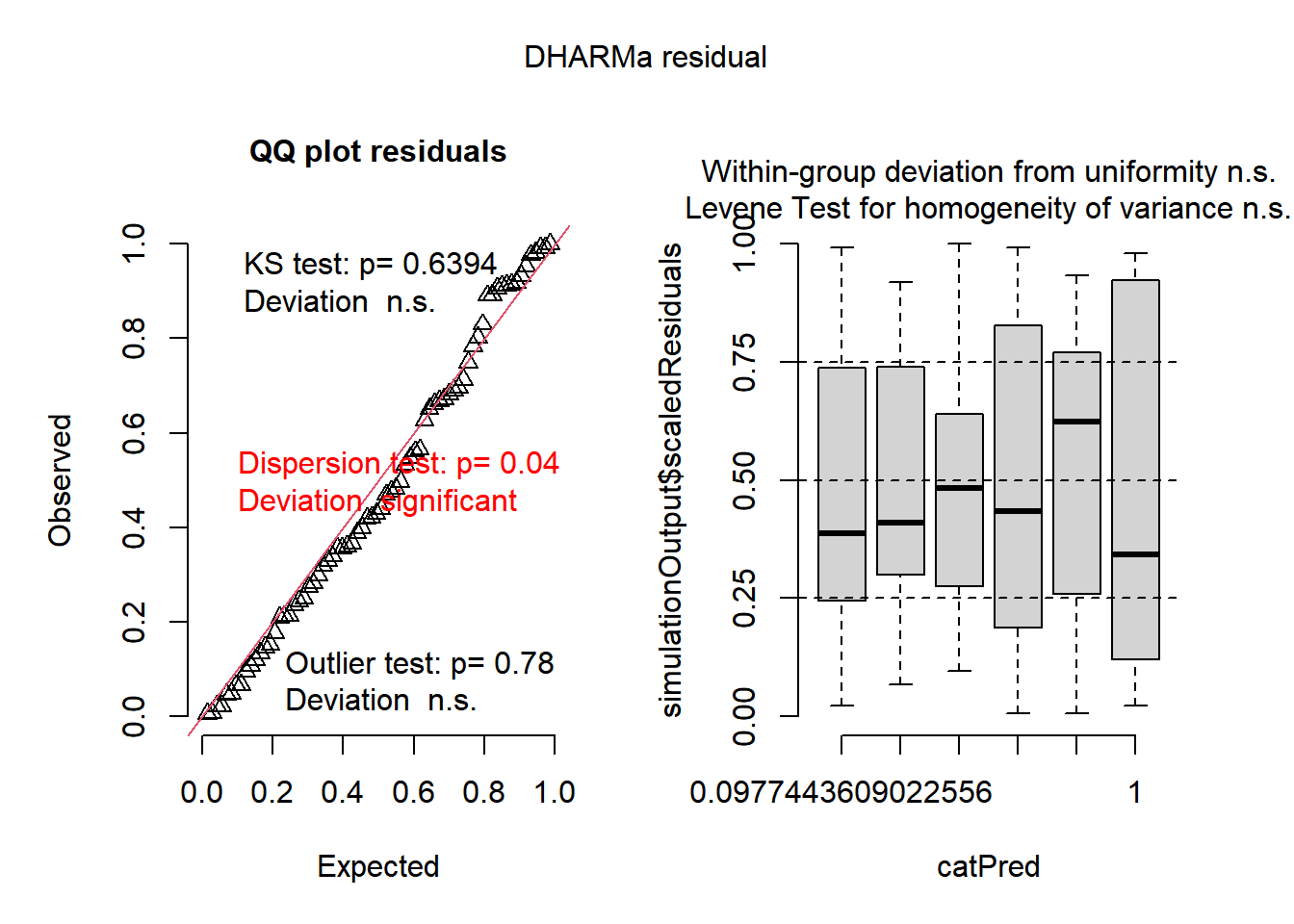
m4 = glm(count ~ spray, data = InsectsDataframe, family = poisson)
plot(simulateResiduals(m4))

mediasM4 = emmeans(m4, ~ spray, type = "response")
cld(mediasM4)

 spray  rate    SE  df asymp.LCL asymp.UCL .group
 C      2.08 0.417 Inf      1.41      3.08  1    
 E      3.50 0.540 Inf      2.59      4.74  12   
 D      4.92 0.640 Inf      3.81      6.35   2   
 A     14.50 1.100 Inf     12.50     16.82    3  
 B     15.33 1.130 Inf     13.27     17.72    3  
 F     16.67 1.180 Inf     14.51     19.14    3  

Confidence level used: 0.95 
Intervals are back-transformed from the log scale 
P value adjustment: tukey method for comparing a family of 6 estimates 
Tests are performed on the log scale 
significance level used: alpha = 0.05 
NOTE: If two or more means share the same grouping symbol,
      then we cannot show them to be different.
      But we also did not show them to be the same.

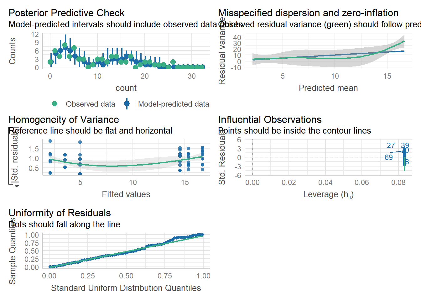
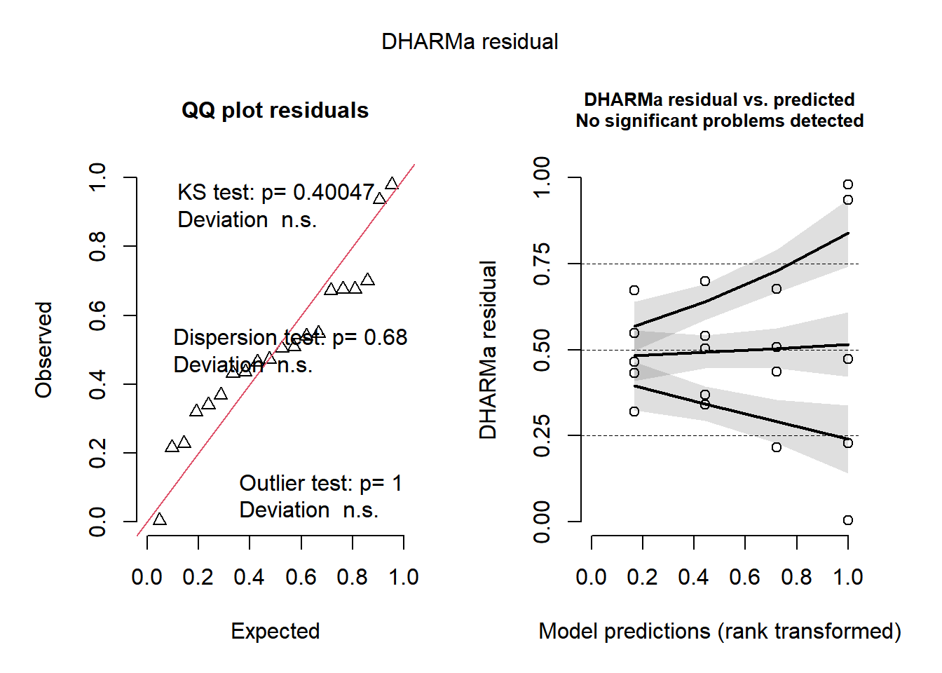
check_model(m4)

ANOVA Fatorial com Interação (Fungicidas)

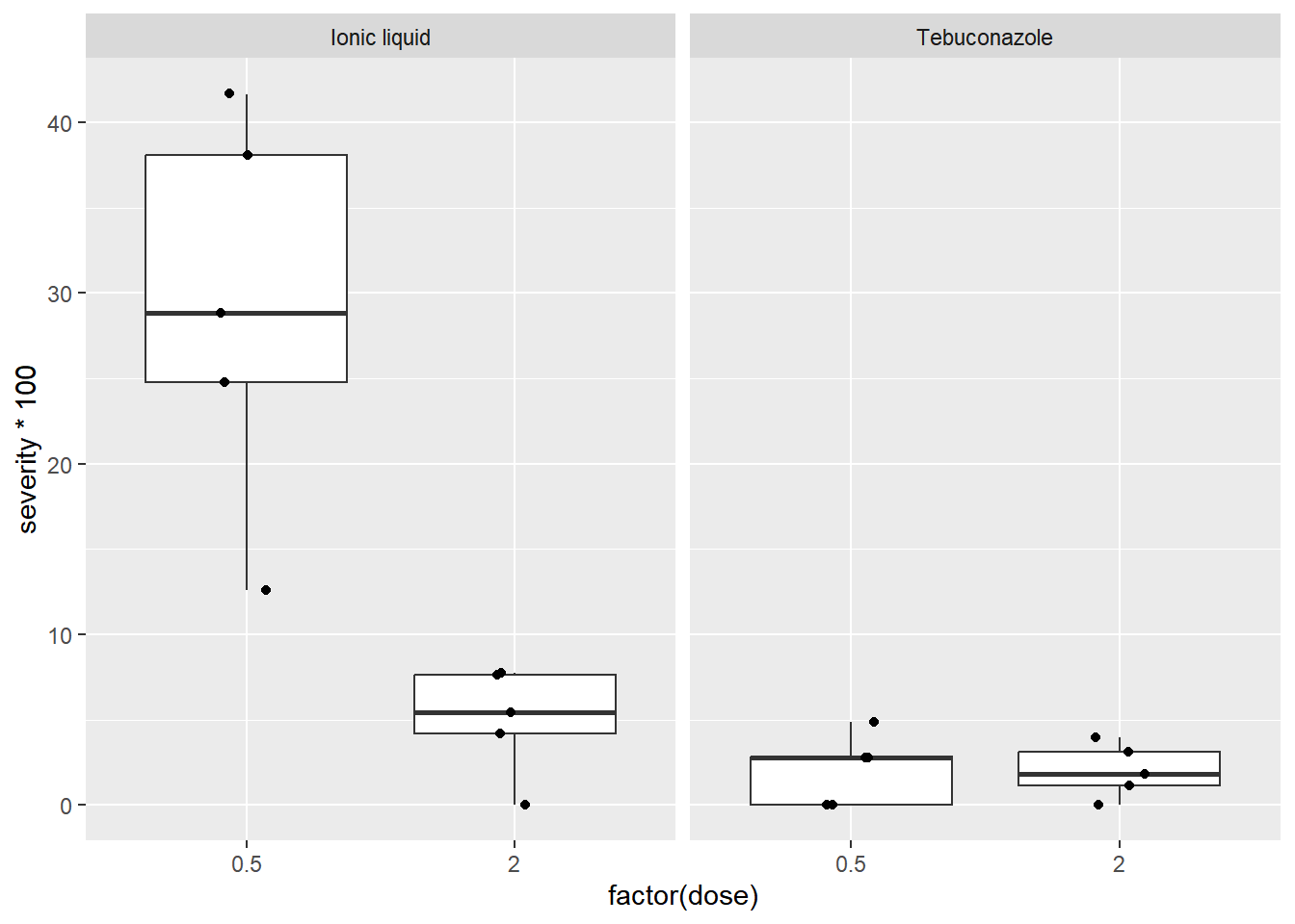
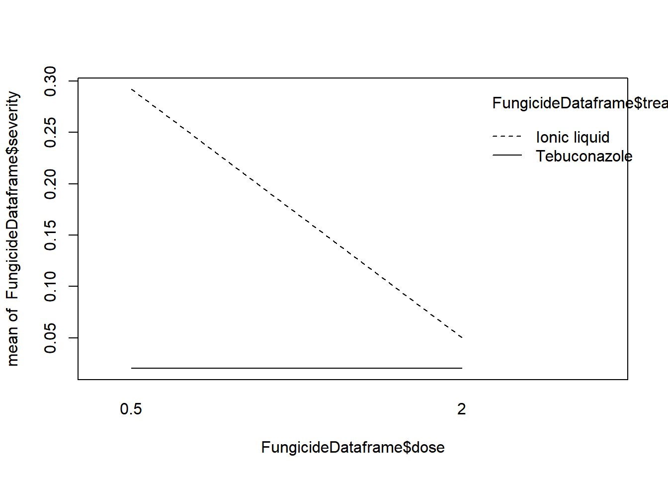
FungicideDataframe = gsheet2tbl("https://docs.google.com/spreadsheets/d/1bq2N19DcZdtax2fQW9OHSGMR0X2__Z9T/edit?gid=2023059672")

# Boxplot por dose e tratamento
FungicideDataframe |>
  ggplot(aes(factor(dose), severity*100)) +
  geom_boxplot(outlier.color = NA) +
  geom_jitter(width = 0.1) +
  facet_wrap(~treat)

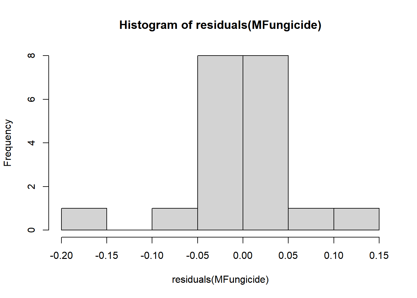
MFungicide = lm(severity ~ treat * dose, data = FungicideDataframe)
hist(residuals(MFungicide))

plot(simulateResiduals(MFungicide))

interaction.plot(FungicideDataframe$dose, FungicideDataframe$treat, FungicideDataframe$severity)

anova(MFungicide)

Analysis of Variance Table

Response: severity
           Df   Sum Sq  Mean Sq F value    Pr(>F)    
treat       1 0.113232 0.113232  30.358 4.754e-05 ***
dose        1 0.073683 0.073683  19.755 0.0004077 ***
treat:dose  1 0.072739 0.072739  19.502 0.0004326 ***
Residuals  16 0.059678 0.003730                      
---
Signif. codes:  0 '***' 0.001 '**' 0.01 '*' 0.05 '.' 0.1 ' ' 1

MediasFungicideByDose = emmeans(MFungicide, ~ treat | dose)
cld(MediasFungicideByDose, Letters = letters)

dose = 0.5:
 treat        emmean     SE df lower.CL upper.CL .group
 Tebuconazole 0.0210 0.0273 16 -0.03690   0.0789  a    
 Ionic liquid 0.2921 0.0273 16  0.23420   0.3500   b   

dose = 2.0:
 treat        emmean     SE df lower.CL upper.CL .group
 Tebuconazole 0.0202 0.0273 16 -0.03768   0.0781  a    
 Ionic liquid 0.0501 0.0273 16 -0.00781   0.1080  a    

Confidence level used: 0.95 
significance level used: alpha = 0.05 
NOTE: If two or more means share the same grouping symbol,
      then we cannot show them to be different.
      But we also did not show them to be the same.

MediasFungicideByTreat = emmeans(MFungicide, ~ dose | treat)
cld(MediasFungicideByTreat, Letters = letters)

treat = Ionic liquid:
 dose emmean     SE df lower.CL upper.CL .group
  2.0 0.0501 0.0273 16 -0.00781   0.1080  a    
  0.5 0.2921 0.0273 16  0.23420   0.3500   b   

treat = Tebuconazole:
 dose emmean     SE df lower.CL upper.CL .group
  2.0 0.0202 0.0273 16 -0.03768   0.0781  a    
  0.5 0.0210 0.0273 16 -0.03690   0.0789  a    

Confidence level used: 0.95 
significance level used: alpha = 0.05 
NOTE: If two or more means share the same grouping symbol,
      then we cannot show them to be different.
      But we also did not show them to be the same.

cv.model(MFungicide)

[1] 63.7165

AUDPC e Interação Fatorial (Oídio)

MildewDataframe = PowderyMildew |> 
  filter(irrigation_type %in% c("MS", "MS above canopy", "Overhead"))

MildewDataframe |>
  ggplot(aes(time, sev*100)) +
  geom_jitter(width = 0.1) +
  facet_grid(moisture ~ irrigation_type)

MildewDataframeAUDPC = MildewDataframe |>
  group_by(irrigation_type, moisture, block) |>
  summarise(AUDPC = AUDPC(time, sev), .groups = "drop")

ggplot(MildewDataframeAUDPC, aes(irrigation_type, AUDPC, color = moisture)) +
  geom_jitter(width = 0.1)

MMildew = lm(AUDPC ~ irrigation_type * moisture, data = MildewDataframeAUDPC)
hist(residuals(MMildew))

plot(simulateResiduals(MMildew))

interaction.plot(MildewDataframeAUDPC$irrigation_type, MildewDataframeAUDPC$moisture, MildewDataframeAUDPC$AUDPC)

anova(MMildew)

Analysis of Variance Table

Response: AUDPC
                         Df  Sum Sq Mean Sq F value    Pr(>F)    
irrigation_type           2 134.341  67.170 451.721 5.073e-12 ***
moisture                  1   6.680   6.680  44.924 2.188e-05 ***
irrigation_type:moisture  2   5.104   2.552  17.162 0.0003022 ***
Residuals                12   1.784   0.149                      
---
Signif. codes:  0 '***' 0.001 '**' 0.01 '*' 0.05 '.' 0.1 ' ' 1

MediasMildewByMoisture = emmeans(MMildew, ~ irrigation_type | moisture)
cld(MediasMildewByMoisture, Letters = letters)

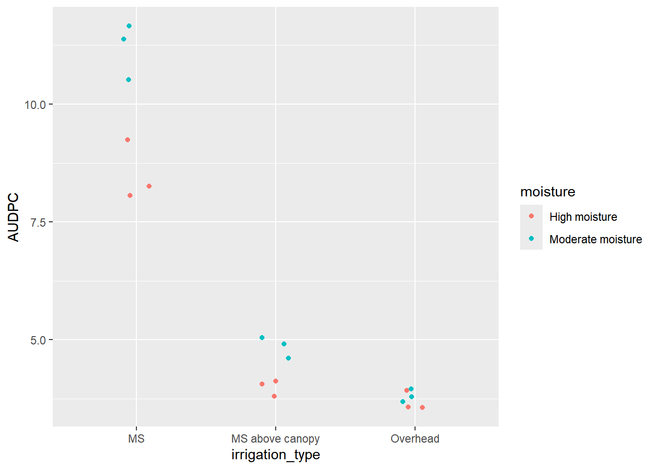
moisture = High moisture:
 irrigation_type emmean    SE df lower.CL upper.CL .group
 Overhead          3.68 0.223 12     3.20     4.17  a    
 MS above canopy   3.99 0.223 12     3.51     4.48  a    
 MS                8.52 0.223 12     8.04     9.01   b   

moisture = Moderate moisture:
 irrigation_type emmean    SE df lower.CL upper.CL .group
 Overhead          3.81 0.223 12     3.33     4.30  a    
 MS above canopy   4.86 0.223 12     4.37     5.34   b   
 MS               11.18 0.223 12    10.70    11.67    c  

Confidence level used: 0.95 
P value adjustment: tukey method for comparing a family of 3 estimates 
significance level used: alpha = 0.05 
NOTE: If two or more means share the same grouping symbol,
      then we cannot show them to be different.
      But we also did not show them to be the same.

MediasMildewByIrrigationType = emmeans(MMildew, ~ moisture | irrigation_type)
cld(MediasMildewByIrrigationType, Letters = letters)

irrigation_type = MS:
 moisture          emmean    SE df lower.CL upper.CL .group
 High moisture       8.52 0.223 12     8.04     9.01  a    
 Moderate moisture  11.18 0.223 12    10.70    11.67   b   

irrigation_type = MS above canopy:
 moisture          emmean    SE df lower.CL upper.CL .group
 High moisture       3.99 0.223 12     3.51     4.48  a    
 Moderate moisture   4.86 0.223 12     4.37     5.34   b   

irrigation_type = Overhead:
 moisture          emmean    SE df lower.CL upper.CL .group
 High moisture       3.68 0.223 12     3.20     4.17  a    
 Moderate moisture   3.81 0.223 12     3.33     4.30  a    

Confidence level used: 0.95 
significance level used: alpha = 0.05 
NOTE: If two or more means share the same grouping symbol,
      then we cannot show them to be different.
      But we also did not show them to be the same.

cv.model(MMildew)

[1] 6.418205