aula_3 – <i class='bi bi-graph-up'></i> FIP 606

O que aprendemos?

1. Teste t para Amostras Independentes

Quando utilizar: comparar médias entre dois grupos distintos (ex: tratamento vs. controle)
Verificação de premissas: normalidade (teste de Shapiro-Wilk) e homogeneidade de variâncias (teste F)
Utilização da função t.test() com var.equal = FALSE para caso variâncias diferentes
Visualização com ggboxplot() e adição de valor-p com stat_pvalue_manual()

2. Teste t para Amostras Dependentes (Pareado)

Quando utilizar: comparação antes e depois no mesmo indivíduo (ex: Unaided vs Aided1)
Uso da função t.test(..., paired = TRUE)
Exploração de normalidade e variância com shapiro.test() e var.test()
Alternativas não-paramétricas: wilcox.test() (teste de Wilcoxon)

3. ANOVA (Análise de Variância)

Quando utilizar: comparação entre três ou mais grupos (ex: espécies de fungos)
Verificação de premissas: normalidade dos resíduos, homogeneidade das variâncias (bartlett.test, levene_test)
Comparações múltiplas com emmeans, pairs() e cld()
Visualização de grupos com ggplot2

4. Testes para Dados Não-Normais ou Variância Desigual

Transformações da variável resposta: log(), sqrt(), rank() (com cuidado!)
Alternativa não-paramétrica à ANOVA: Kruskal-Wallis com kruskal.test()
Comparações múltiplas para Kruskal com pacote agricolae

Teste t para Amostras Independentes

dat_mg <- gsheet2tbl("https://docs.google.com/spreadsheets/d/1bq2N19DcZdtax2fQW9OHSGMR0X2__Z9T/edit?gid=983033137")

ggplot(dat_mg, aes(trat, comp)) +
  geom_jitter(width = 0.1)

dat_mg2 <- dat_mg |>
  pivot_wider(names_from = trat, values_from = comp)

t_results <- t.test(dat_mg2$control, dat_mg2$Mg2, var.equal = FALSE)
report(t_results)

Effect sizes were labelled following Cohen's (1988) recommendations.

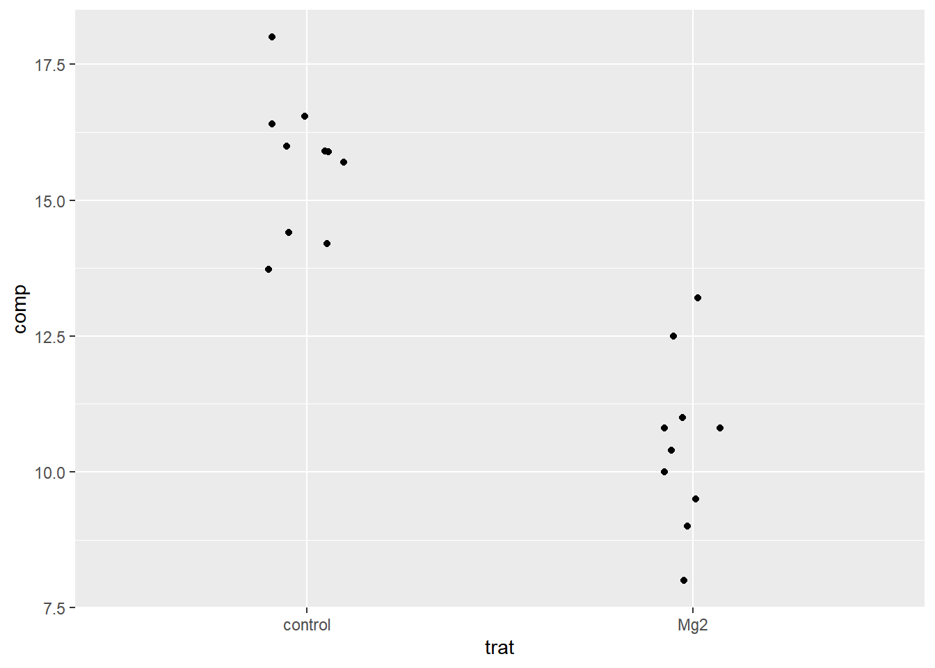
The Welch Two Sample t-test testing the difference between dat_mg2$control and
dat_mg2$Mg2 (mean of x = 15.68, mean of y = 10.52) suggests that the effect is
positive, statistically significant, and large (difference = 5.16, 95% CI
[3.83, 6.49], t(17.35) = 8.15, p < .001; Cohen's d = 3.65, 95% CI [2.14, 5.12])

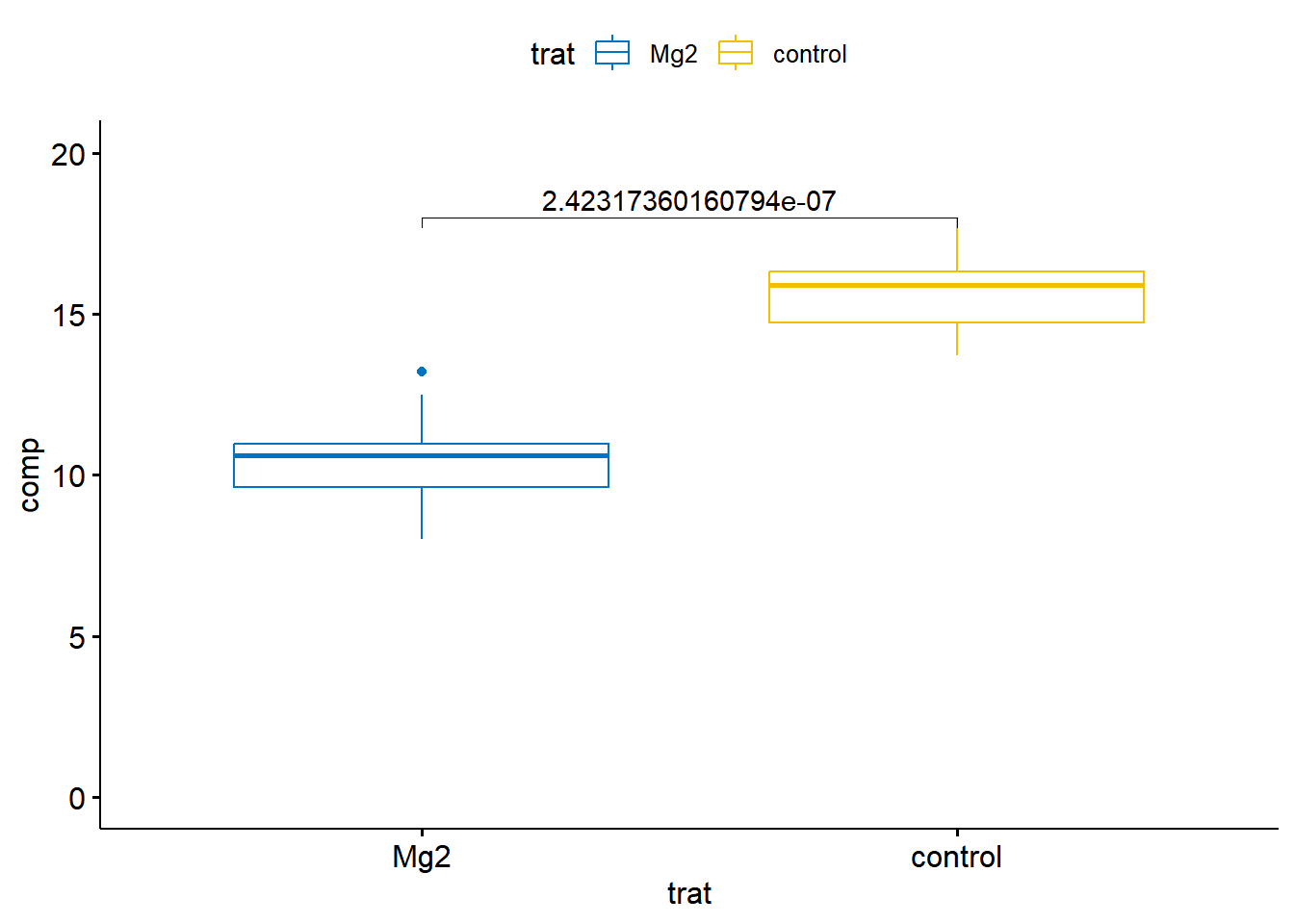
p <- ggboxplot(dat_mg, x = "trat", y = "comp", color = "trat", palette = "jco")
test_df <- data.frame(group1 = "control", group2 = "Mg2", p.value = t_results$p.value, y.position = 18)
p + stat_pvalue_manual(test_df, label = "p.value") + ylim(0, 20)

shapiro.test(dat_mg2$Mg2)


    Shapiro-Wilk normality test

data:  dat_mg2$Mg2
W = 0.97269, p-value = 0.9146

shapiro.test(dat_mg2$control)


    Shapiro-Wilk normality test

data:  dat_mg2$control
W = 0.93886, p-value = 0.5404

var.test(dat_mg2$Mg2, dat_mg2$control)


    F test to compare two variances

data:  dat_mg2$Mg2 and dat_mg2$control
F = 1.4781, num df = 9, denom df = 9, p-value = 0.5698
alternative hypothesis: true ratio of variances is not equal to 1
95 percent confidence interval:
 0.3671417 5.9508644
sample estimates:
ratio of variances 
          1.478111

Teste t para Amostras Dependentes

escala <- gsheet2tbl("https://docs.google.com/spreadsheets/d/1bq2N19DcZdtax2fQW9OHSGMR0X2__Z9T/edit?gid=1729131173")

escala_wider <- escala |> pivot_wider(id_cols = rater, names_from = assessment, values_from = acuracia)

t.test(escala_wider$Unaided, escala_wider$Aided1, paired = TRUE)


    Paired t-test

data:  escala_wider$Unaided and escala_wider$Aided1
t = -4.4214, df = 9, p-value = 0.001668
alternative hypothesis: true mean difference is not equal to 0
95 percent confidence interval:
 -0.3552353 -0.1147647
sample estimates:
mean difference 
         -0.235

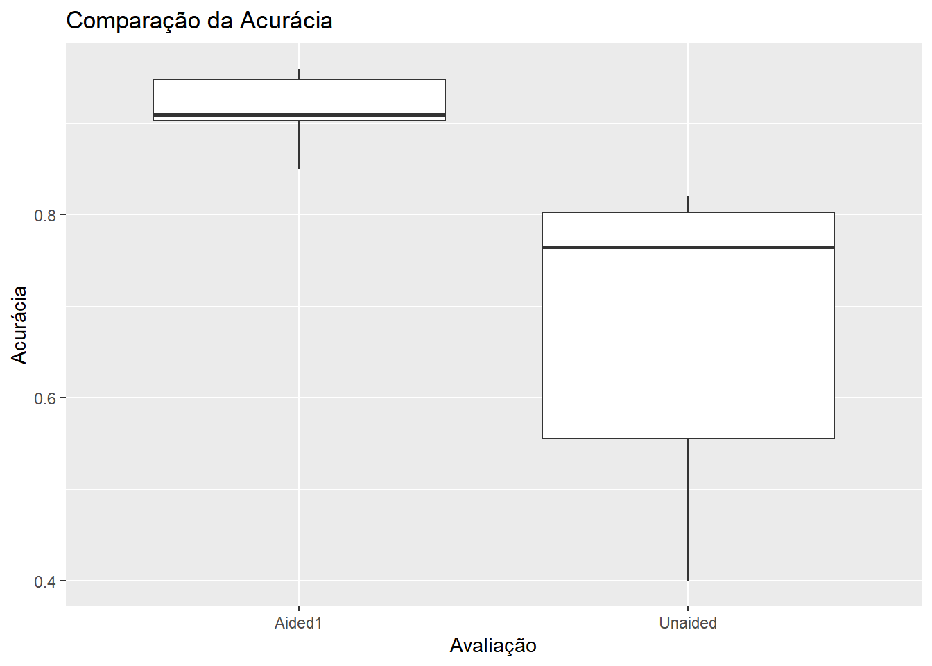
ggplot(escala, aes(x = assessment, y = acuracia)) +
  geom_boxplot() +
  labs(title = "Comparação da Acurácia", x = "Avaliação", y = "Acurácia")

unaided <- escala |> filter(assessment == "Unaided") |> pull(acuracia)
aided <- escala |> filter(assessment == "Aided1") |> pull(acuracia)
var.test(unaided, aided)


    F test to compare two variances

data:  unaided and aided
F = 20.978, num df = 9, denom df = 9, p-value = 0.000106
alternative hypothesis: true ratio of variances is not equal to 1
95 percent confidence interval:
  5.210754 84.459185
sample estimates:
ratio of variances 
          20.97847

shapiro.test(unaided)


    Shapiro-Wilk normality test

data:  unaided
W = 0.7748, p-value = 0.007155

shapiro.test(aided)


    Shapiro-Wilk normality test

data:  aided
W = 0.92852, p-value = 0.4335

wilcox.test(unaided, aided, paired = TRUE)


    Wilcoxon signed rank test with continuity correction

data:  unaided and aided
V = 0, p-value = 0.005889
alternative hypothesis: true location shift is not equal to 0

ANOVA - Crescimento Micelial

micelial <- gsheet2tbl("https://docs.google.com/spreadsheets/d/1bq2N19DcZdtax2fQW9OHSGMR0X2__Z9T/edit?gid=959387827")

ggplot(micelial, aes(x = especie, y = tcm)) +
  geom_boxplot() +
  geom_jitter(width = 0.1)

anova1 <- aov(tcm ~ especie, data = micelial)
shapiro.test(residuals(anova1))


    Shapiro-Wilk normality test

data:  residuals(anova1)
W = 0.9821, p-value = 0.8782

bartlett.test(tcm ~ especie, data = micelial)


    Bartlett test of homogeneity of variances

data:  tcm by especie
Bartlett's K-squared = 4.4367, df = 4, p-value = 0.3501

levene_test(tcm ~ especie, data = micelial)

# A tibble: 1 × 4
    df1   df2 statistic     p
  <int> <int>     <dbl> <dbl>
1     4    25      1.76 0.169

m <- emmeans(anova1, ~ especie)
pairs(m)

 contrast    estimate    SE df t.ratio p.value
 Fasi - Faus    0.335 0.079 25   4.241  0.0023
 Fasi - Fcor    0.250 0.079 25   3.165  0.0302
 Fasi - Fgra    0.660 0.079 25   8.356  <.0001
 Fasi - Fmer    0.145 0.079 25   1.836  0.3765
 Faus - Fcor   -0.085 0.079 25  -1.076  0.8169
 Faus - Fgra    0.325 0.079 25   4.115  0.0031
 Faus - Fmer   -0.190 0.079 25  -2.405  0.1469
 Fcor - Fgra    0.410 0.079 25   5.191  0.0002
 Fcor - Fmer   -0.105 0.079 25  -1.329  0.6761
 Fgra - Fmer   -0.515 0.079 25  -6.520  <.0001

P value adjustment: tukey method for comparing a family of 5 estimates

cld(m)

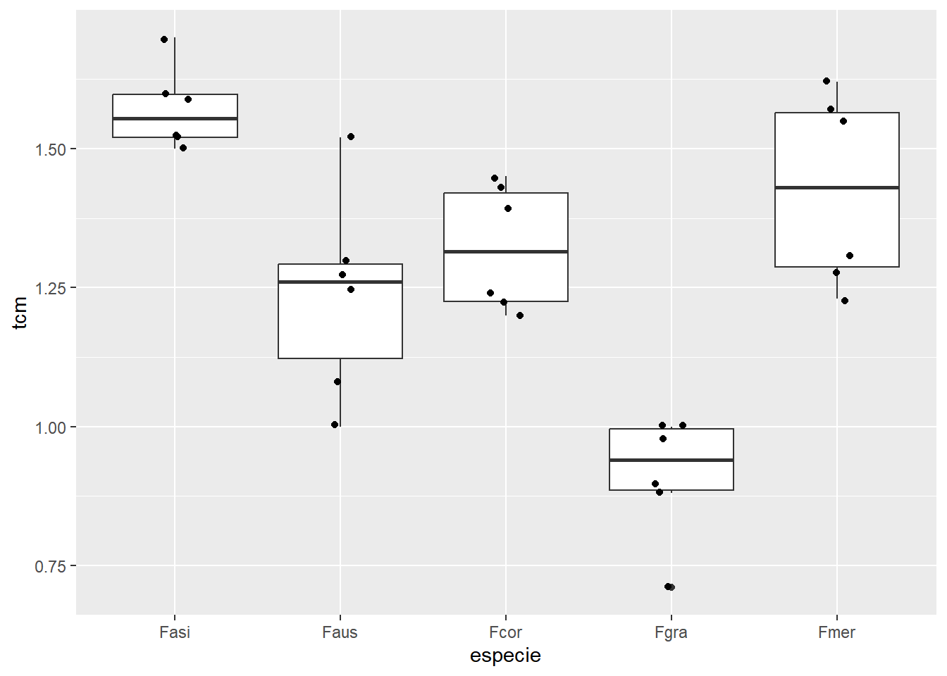
 especie emmean     SE df lower.CL upper.CL .group
 Fgra     0.912 0.0559 25    0.797     1.03  1    
 Faus     1.237 0.0559 25    1.122     1.35   2   
 Fcor     1.322 0.0559 25    1.207     1.44   2   
 Fmer     1.427 0.0559 25    1.312     1.54   23  
 Fasi     1.572 0.0559 25    1.457     1.69    3  

Confidence level used: 0.95 
P value adjustment: tukey method for comparing a family of 5 estimates 
significance level used: alpha = 0.05 
NOTE: If two or more means share the same grouping symbol,
      then we cannot show them to be different.
      But we also did not show them to be the same.

Kruskal-Wallis e Alternativas

insetos <- InsectSprays

ggplot(insetos, aes(x = spray, y = count)) +
  geom_boxplot() +
  geom_jitter(width = 0.1)

kruskal.test(count ~ spray, data = insetos)


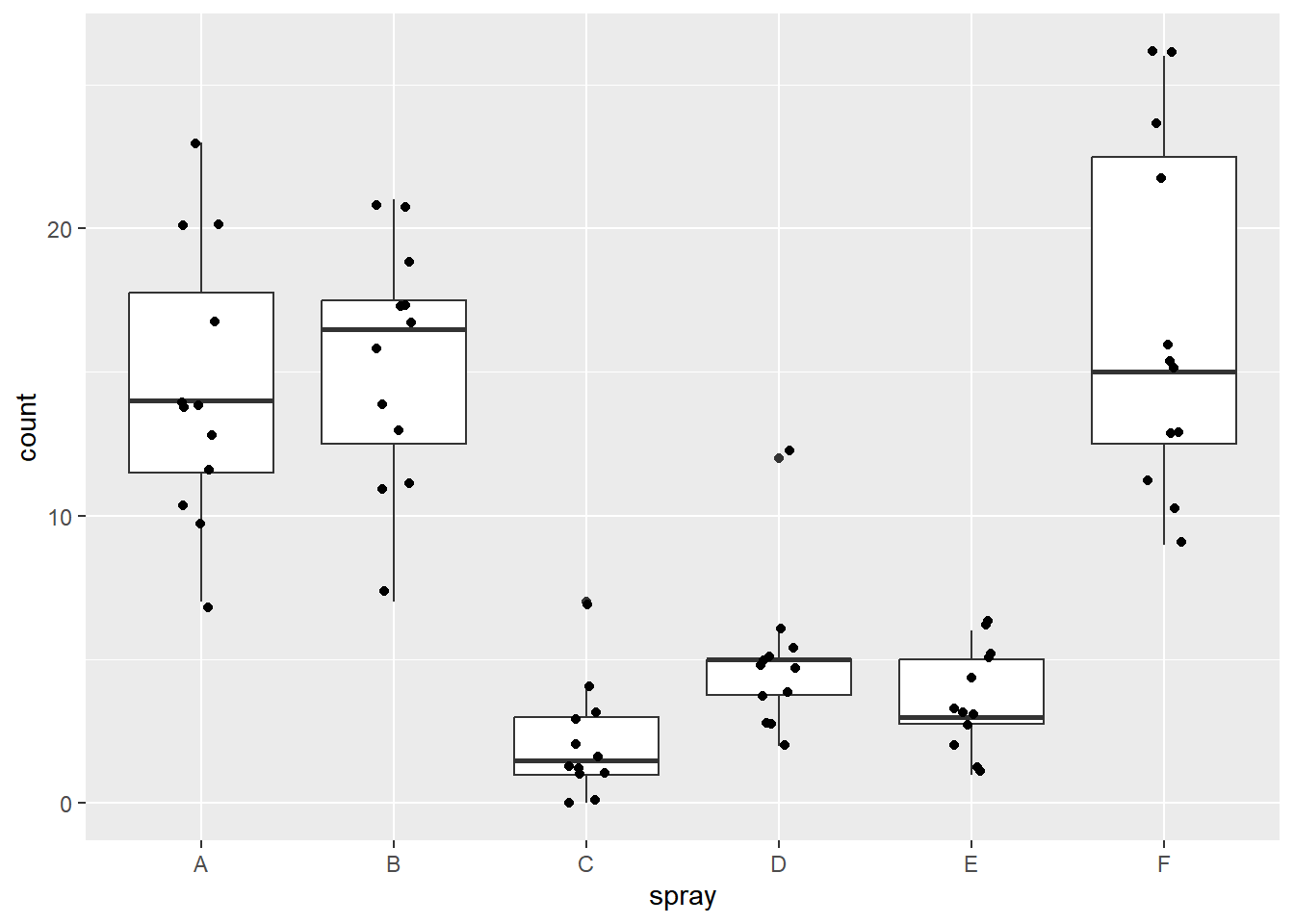
    Kruskal-Wallis rank sum test

data:  count by spray
Kruskal-Wallis chi-squared = 54.691, df = 5, p-value = 1.511e-10

kruskal.out <- with(insetos, kruskal(count, spray, group = TRUE, console = TRUE))


Study: count ~ spray
Kruskal-Wallis test's
Ties or no Ties

Critical Value: 54.69134
Degrees of freedom: 5
Pvalue Chisq  : 1.510845e-10 

spray,  means of the ranks

     count  r
A 52.16667 12
B 54.83333 12
C 11.45833 12
D 25.58333 12
E 19.33333 12
F 55.62500 12

Post Hoc Analysis

t-Student: 1.996564
Alpha    : 0.05
Minimum Significant Difference: 8.462804 

Treatments with the same letter are not significantly different.

     count groups
F 55.62500      a
B 54.83333      a
A 52.16667      a
D 25.58333      b
E 19.33333     bc
C 11.45833      c

print(kruskal.out)

$statistics
     Chisq Df      p.chisq  t.value      MSD
  54.69134  5 1.510845e-10 1.996564 8.462804

$parameters
            test p.ajusted name.t ntr alpha
  Kruskal-Wallis      none  spray   6  0.05

$means
      count     rank      std  r Min Max   Q25  Q50   Q75
A 14.500000 52.16667 4.719399 12   7  23 11.50 14.0 17.75
B 15.333333 54.83333 4.271115 12   7  21 12.50 16.5 17.50
C  2.083333 11.45833 1.975225 12   0   7  1.00  1.5  3.00
D  4.916667 25.58333 2.503028 12   2  12  3.75  5.0  5.00
E  3.500000 19.33333 1.732051 12   1   6  2.75  3.0  5.00
F 16.666667 55.62500 6.213378 12   9  26 12.50 15.0 22.50

$comparison
NULL

$groups
     count groups
F 55.62500      a
B 54.83333      a
A 52.16667      a
D 25.58333      b
E 19.33333     bc
C 11.45833      c

attr(,"class")
[1] "group"

Dicas Finais

Use paired = TRUE para medidas repetidas.
Use var.equal = FALSE como padrão no t.test() se as variâncias forem diferentes.
Testes não-paramétricos (Wilcoxon, Kruskal) são bons aliados quando as premissas não são atendidas.
Visualize sempre os dados antes de aplicar testes!